Parallel Radix Sort Algorithm Using Message Passing Interface (MPI)

MPI is a Standardized and Portable Message-Passing Standard Designed to Function on Parallel Computing Architectures

In one of our earlier articles, we’ve discussed the Radix Sort algorithm and its implementation along with its features in a brief.

We didn’t discuss the Parallelizability of Radix Sort in that article and we’re going to discuss it here.

The key theory behind a radix sort is to sort each component digit by digit, from least significant to most substantial. We will arrange the elements so that the digits are in ascending order for each digit.

For the original string set and large subsets, we use a fully parallel radix sort, a sequential radix sort for medium-sized subsets, and an insertion sort for base cases. A counting phase, a global prefix sum, and a redistribution step comprise a fully parallel radix sort.

Image Source: https://hpc.ipm.ac.ir/2019/01/13/mpi/

Parallel sorting is a crucial part of parallel computing. It enables us to minimize sorting time and sort larger amounts of data that cannot be sorted serially. Whenever we want to sort a large amount of data, it is possible that it will not fit on a single computer because computers have limited memory.

Alternatively, using only one computer may take too much time, which we cannot afford. One of those that meet our requirements while remaining efficient is the parallel Radix Sort. It is currently recognized as the most efficient internal sorting method for distributed-memory multiprocessors.

In general, parallel sorts consist of various rounds of the serial sort, known as local sort, performed in parallel by each processor, followed by key mobility among processors, known as the redistribution step. Based on the algorithms used, local sort and data redistribution may be interleaved and iterated several times. This pattern is also followed by the parallel Radix Sort.

We assume that each processor has almost the same amount of data; alternatively, the workload of the processors would be unbalanced due to the local sort. Indeed, if one processor has much more data than the others, it will take longer to complete its local sort, resulting in a longer total sorting time.

However, if the data is evenly distributed, all of the processors will take the same amount of time to complete their local sort, and none will have to wait for another to finish. As a result, the overall sorting time will be reduced.

The parallel Radix Sort works by first sorting the data on each processor according to the digit value for each key digit. That is done by all of the processors at the same time. Then, determine which processors must send which sections of their local data to which other processors in order to have the distributed list sorted across processors and by digit. The distributed array will be sorted as desired after iterating for the last key digit.

Parallel Radix Sort Algorithm

Input: rank (rank of the processor), L (portion of the distributed data held by this processor)
Output: the distributed data sorted across the processors with the same amount of data for each processor
1. For each keys digit i where i varies from the least significant digit to the most significant digit:
2. Use Counting Sort or Bucket Sort to sort L according to the i th keys digit
3. Share information with other processors to figure out which local data to send where and what to receive from which processors in order to have the distributed array sorted across processors according to the i th keys digit
4. Proceed to these exchanges of data between processors

Each processor executes the algorithm with its own rank and share of the distributed data. This is a parallel Radix Sort algorithm at a high level. It defines what to do but not how to do it because there are numerous ways to carry out steps 3 and 4 based on a variety of factors such as the architecture, environment, and communication tool used. Let’s look at an example.

Parallel Radix Implementation

1. Divide the data to all other processors if it is originally present in a single processor.
2. Convert the numbers to base 2 notation (Binary). We went from Least Significant Digit to Most Significant Digit in base 10.
3. Carry out an interprocess communication.
4. On these processors, perform a counting sort locally.
5. Calculate the global prefix-sum of each processor’s integer count.
6. Using the index calculated in the previous step, put the integers back into a temporary array that will be used as input for the next iteration.

For the parallel implementation, we choose a group of g bits. If p = Number of processors. Then we choose g such that,

2ᵍ = p

g = log₂P

For example, if p = 4, then g = 2. We take 2 bits at a time 00, 01, 10, 11.

Implementation explanation

Let’s sort the following set of numbers using 3 processors with 15 numbers to sort. That is; P=3, N=15.

27, 13, 18, 99, 02, 75, 14, 26, 29, 05, 25, 49, 53, 61, 03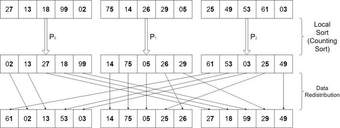

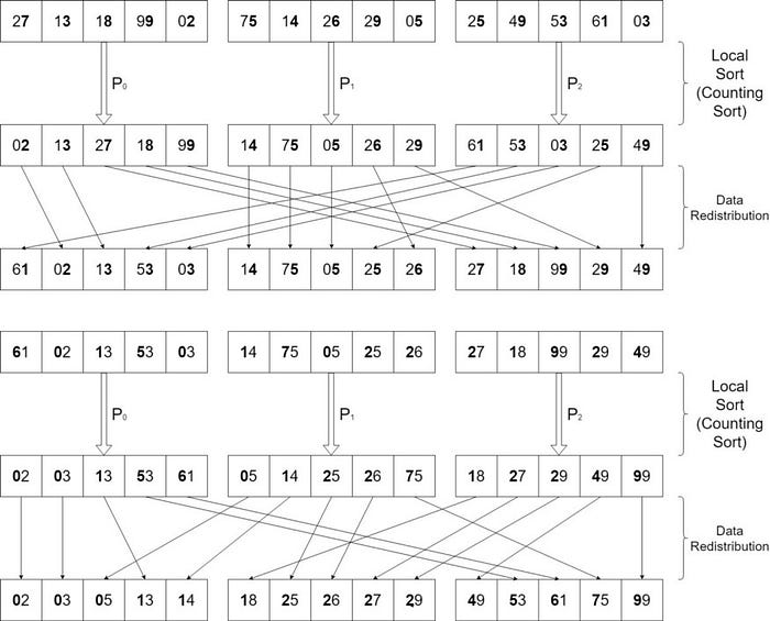
Image by Author: LSD based Parallel Radix Sort

The numbers are sorted by their base 10 LSD (Least Significant Digit). The first step (local sorting) is performed simultaneously by all processors. Depending on the architecture, environment, and communication tool used, the second step (data redistribution) can be computed and managed in a variety of ways. It takes one iteration based on their base 10 MSD to complete the algorithm and obtain the desired final distributed sorted array.

If we exchange the local sort step and the data redistribution step, the algorithm remains correct. However, in practice, it is insufficient because, in order to send data efficiently, the data must be contiguous in memory. Because two data sets with the same ith digit will almost certainly be sent to the same processor, it is a good idea to sort the data locally first.

As per the algorithm, we still have one iteration to go. Let’s wrap this up.

Image by Author: MSD based Parallel Radix Sort

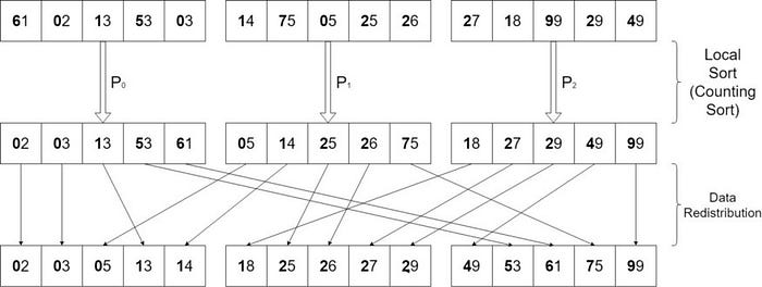
The numbers are sorted by their base 10 MSD (Most Significant Digit). The first step (local sorting) is performed simultaneously by all processors. Depending on the architecture, environment, and communication tools used, the second step (data redistribution) can be computed and managed in a variety of ways. Finally, the algorithm is finished, and the distributed array is sorted.

MPI is a protocol that allows processors to communicate with one another. I used the Counting Sort rather than the Bucket Sort because my implementation with the Bucket Sort had a memory management cost. Indeed, unless we do the first loop through the keys to count them before moving them into the buckets, we don’t know the length of the buckets in advance.

To execute step 3 of the algorithm, we can save the local counts from the Counting Sort on each processor and distribute them to other processors. As a result, each processor knows how many keys on each processor have their ith byte equal to a given value, and it is simple to figure out where to send which data as explained above in images.

Step 4 is handled using one-sided MPI communications rather than two-sided send and receive communications as the results were comparable or better with one-sided communications on many occasions. When the hardware supports RMA operations, MPI one-sided communications are more efficient. We can use them in step 4 of parallel Radix Sort because we don’t need synchronization for each data movement, only when they’re all finished.

In step 4, the data movements are completely independent; they can be performed in any order as long as we know where each element must go.

Image by Author: Implementation

Try to implement this in C or any preferred Programming Language and let me know.

Hope this article can help. Share your thoughts too.